Introduction
This is an implementation of Neural Texture Compression (NTC) which is based on the NVIDIA research paper: Random-Access Neural Compression of Material Textures. I was at the point where I wanted to do texture compression for my custom engine, and after skimming through this research, I was impressed with the compression-quality results. So I went down the rabbit hole of machine learning.
This post will serve as extended documentation of MetalNTC. It focuses on the details that decide performance and visual fidelity when NTC has to work inside a Metal renderer. I will discuss positives/negatives and fail cases, as well as use cases of NTC, since for now it can’t entirely replace traditional texture sampling. Moreover, we will see how much the newly added neural accelerators on M5 chip help with real-time inference and latency hiding as well as how NTC can provide value even on an M1 air.
Motivation
Besides NTC’s quality advantage over BCn (Block Compression), as shown in the NVIDIA research, a great motivation for taking this path is the memory/storage shortage and the increasing size of video games. High quality materials take a big part in how a scene looks, and I wouldn’t want VRAM or disk size to be the limit on how good they can look.
Creating the ground truth
The Multilayer Perceptron (MLP) will be able to decompress any texture and mip level of the material texture set. Hence it needs the mips for each one of the source textures. Conveniently, my last post was on a Single Pass Downsampler which I could reuse. The only difference now is that it receives a texture2d_array, and every thread loops over the number of materials the texture set includes.
Training
Forward pass
-
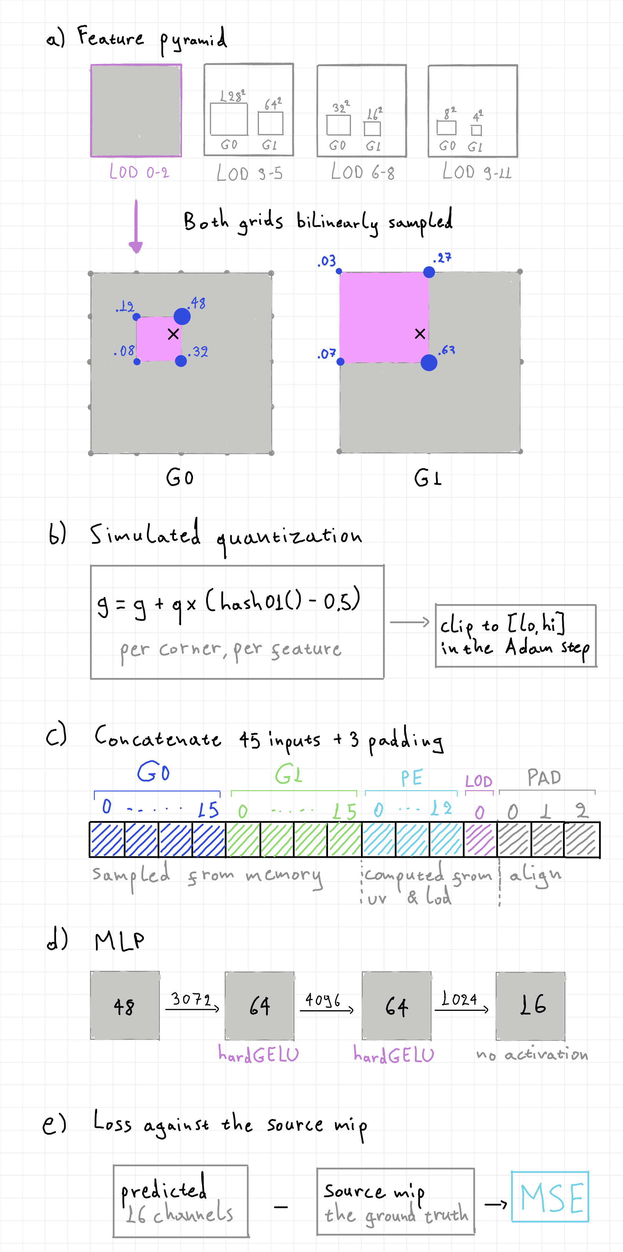
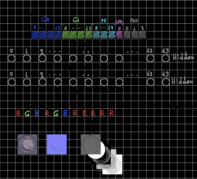
The neural network is using latent grids with learned features. Each mip level is using a pair of latent grids, where this pair can be used by many mip levels. This sharing of features lowers the storage cost of a traditional mipmap chain. The grid G0 is at higher resolution, which helps preserve high frequency details, while G1 is at a lower resolution, helping with the reconstruction of low frequency content. Both of them are bilinearly sampled and their features are later concatenated and not blended. The choice of which grid pair that a mip should use is empirical.
-
During training uniform noise is applied that simulates what would happen if the parameters were quantized. Quantization produces an error that is approximately uniformly distributed, hence the [-q/2, q/2) noise is applied. The actual quantization takes place at a later stage, but the neural network must be trained on the expected precision loss. The
round()in the quantization would create zero gradients during training, since a small nudge does nothing at all. The gradient is multiplied by the chain rule during backpropagation, so the latents would receive nothing and never get trained. -
Concatenation is the process that will construct the input layer of the MLP. As mentioned before, each latent grid’s features are separate from each other and each one has 16.
The positional encoding (PE) gives the network a signal that the grid’s resolution cannot physically encode. For the case of a 2048x2048 texture, the G1 grid at 256x256 (which is the biggest upsampling) is 8 times smaller than the source. One texel in G1 spreads across an 8x8 block of output texels, so within that block the G1 features vary only as a linear blend of the same four stored texels. PE is what varies inside the block.
Each latent grid pair is used for at least 3 texture mips. All 44 other inputs are identical across the mips that latent pair serves, so the network would be handed the same input and asked for three or more different images. The normalized LOD is the only thing that is different.
The padding is needed because the input layer needs to be a multiple of 16 for the tensor ops.
-
The RTXNTC which is the repository of the Nvidia research, is currently using 64-48-32 hidden layers. However I went with their original 64-64 hidden layers as it was simpler to implement and I’m leaving the new design for the future. The hardGELU is a fast piecewise quadratic approximation of the standard GELU activation.
-
Calculate loss against the ground truth. Channels of different textures have different importance. For example the albedo’s error gets a bigger say in how much it drives the update, whereas textures like the displacement map get smaller weight. Because of the fixed number of features per grid, the weights need to favor the textures whose error shows up in the final image.
Backpropagation
After loss, backpropagation runs backwards on the same layers and same weights but transposed. Forward reads 4 corners and produces 1 feature (gather). Backward takes 1 gradient and writes 4 corners (scatter). The size of the batch is 4096. Each thread in the batch is accumulating its gradients in the shared gradient buffer.
Metal doesn’t have float atomics, so integer atomics are used with a scale factor. The layer weights and biases are accumulated by every thread of the batch, but each thread accumulates only the latent features that it touches.
Instead of plain stochastic gradient descent (SGD), the parameters are updated using the Adam stochastic optimizer. The latent grid gradients are very sparse, so there can be cases where a specific texel won’t receive a gradient for many steps and eventually get one contribution from a single thread. Adam stores momentum for every parameter, so an untouched parameter will still keep descending for a number of steps. The squared gradient average helps normalize the learning rate between different parameters. For example MLP weights are hit by all 4096 threads every step, so their accumulated gradients are large unlike latent grid features.
Quantization
Actual quantization happens right after the training (with the simulated noise) has finished. The grids are quantized down to 4 bits per feature, therefore there are 16 representable values.
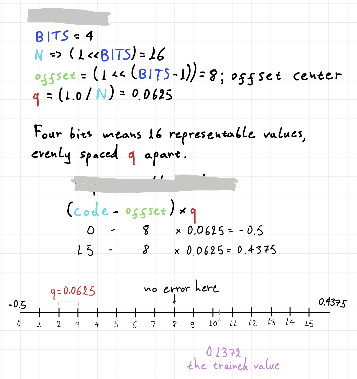
Τhe example below shows the error for the training value 0.1372 as in Figure 2.
Quantization example
| step | expression | result |
|---|---|---|
| trained value | - | 0.1372 |
| scale by 1/q | 0.1372 x 16 |
2.1952 |
| round | rounded() |
2 |
| offset to unsigned | 2 + 8 |
10 |
| clamp | max(0, min(15, 10)) |
10 |
| decode | (10 − 8) x 0.0625 |
0.1250 |
| error | 0.1250 − 0.1372 |
−0.0122 |
Rounding is where precision is lost, but it is necessary for the value to fit in 4bits. Clamping keeps the value inside the bounds (clamping also takes place during the Adam step as in the table below). Decode is using the offset to convert the value from unsigned back to signed and after scaling by q, the error is “decoded - trained value”.
| bound | expression | result |
|---|---|---|
lo |
−(N − 1) / 2 x q = −15/2 x 0.0625 |
−0.46875 |
hi |
N / 2 x q = 16/2 x 0.0625 |
0.5 |
Following the paper, the training runs again for 5% of the original steps, but this time with the decoded latent features frozen. Only the MLP weights are updated to retrain on the rounded latent features.
Inference
Latents as textures
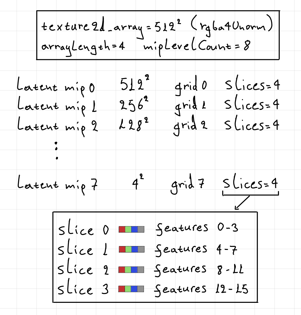
The latent grid features are stored, among others, in the .ntc binary file after the training phase. Since the latent grids will be bilinearly sampled during the inference, the hardware accelerated linear interpolation can be taken advantage of, if the features are stored in textures. However, each latent grid texel is storing 16 features and the rgba4Unorm format (in Metal there is only abgr4Unorm but behaves like rgba4Unorm) can store 4 features. That can be solved by giving each texture 4 slices as seen in Figure 3.
Decoding pixels
The latent grid features are loaded from the .ntc as a texture2d_array and the rest of the MLP weights as a buffer. The rest of the input parameters in Figure 4 are computed and concatenated during runtime. During decoding the forward pass will decode all of the channels in the material texture set, therefore for cases where only a texture needs to be inferred, like in a depth prepass, it is better to use traditional sampling there. The output layer is 16 channels, which should be enough for most of the material texture sets.
Stochastic trilinear interpolation
On current hardware, inference cost is very high even with neural acceleration, and trilinear interpolation to blend mips requires inferring twice. The workaround is to stochastically choose between the mips and accumulate the results across frames.
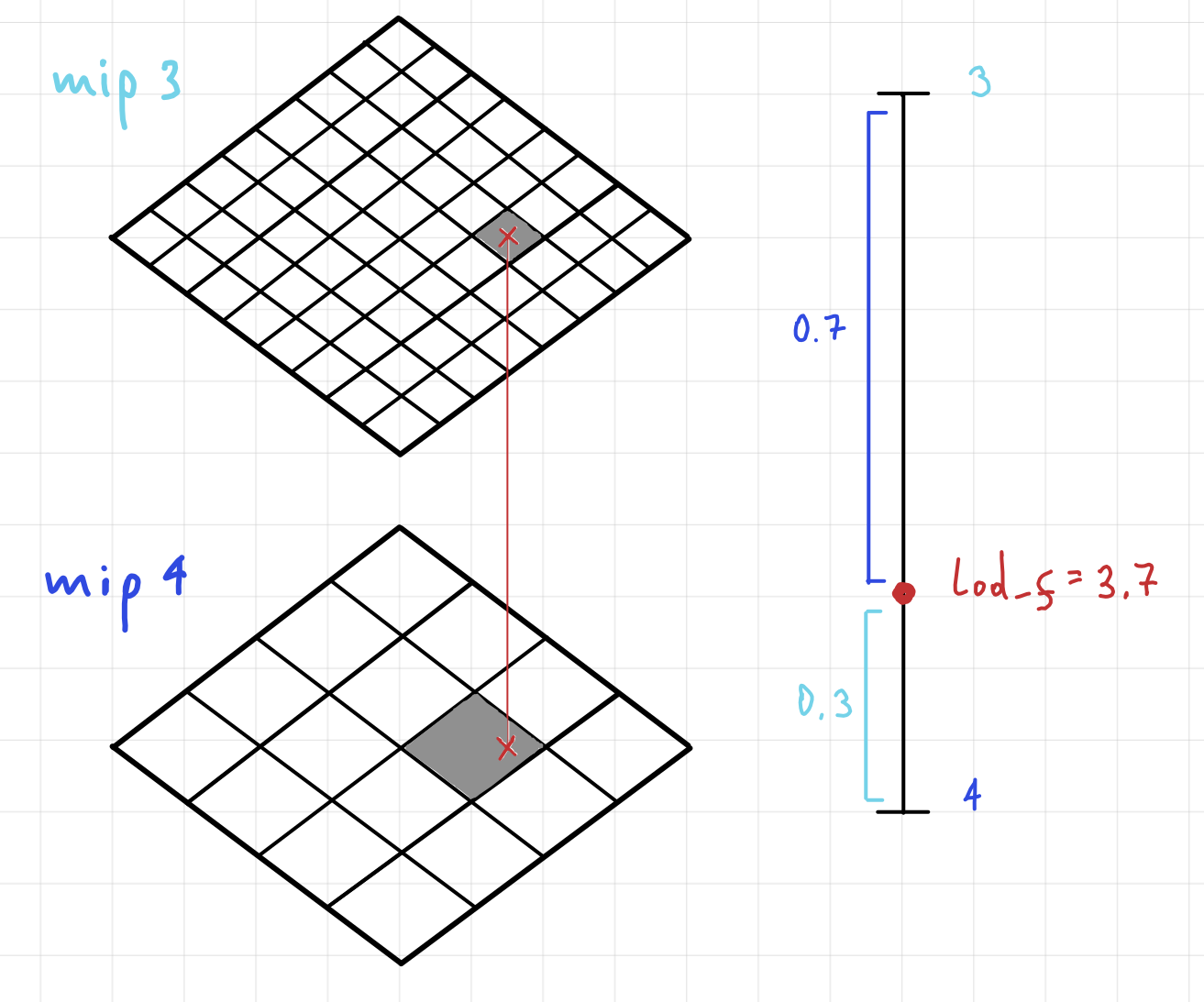
The selection of mip level is calculated in the fragment shader using the dfdx(uv) and dfdy(uv) derivative functions.
| variables | expression | value |
|---|---|---|
| continuous LOD | from dfdx / dfdy |
3.7 |
| base | floor(3.7) |
3 |
| frac | 3.7 − 3 |
0.7 |
| jitter | blue noise, per pixel & frame | [0, 1) |
| chosen mip | jitter < 0.7 ? 4 : 3 |
4 or 3 |
The variable base is used for the base mip level to be inferred and the fractional part is the probability of sampling the base or base + 1 mip level. Jitter varies per pixel using blue noise and per frame using the golden ratio offset. In this example in the table above, mip level 4 has a 70% chance of being inferred on this frame.
Note
In MetalNTC-Renderer a very simple temporal accumulation filter is used just to resolve the shimmering, but in a real application a good TAA solution or similar would be needed.
Optimizations
All the optimization measurements (except tensor ops) took place on the M1 Air 8gb. On a side note, previously were already mentioned optimizations like quantization and hardware accelerated bilinear interpolation. These optimizations are specifically for the forward pass which is the main bottleneck.
Half precision (fp16)
In Apple silicon, using fp16 units is straight forward. This was the lowest hanging fruit in optimizations, as using half floats where possible, proved to improve inference by 90%.
Reducing instruction count
The naive version would load 16 bits where each load would cost one issue slot. Using 64 bits (half4) it reduces the instruction count by 4x. The improvement was 3.08x faster which lands below the theoretical 4x. This makes sense since the horizontal reduce (rowSum), hardGELU, latent sample(), PE and anything PBR related are untouched.
// before: one weight per load
for (uint outNeuron = 0; outNeuron < hidden; outNeuron++) {
    half rowSum = mlp[offset_b1 + outNeuron];
    for (uint i = 0; i < in_dim; i++) {
      rowSum += mlp[offset_w1 + outNeuron * in_dim + i] * features[i];
    }
    hid1[outNeuron] = hard_gelu(rowSum);
}
// pack the padded input vector into aligned half4 groups
half4 input4[F_IN / 4];
for (uint group = 0; group < in_dim / 4; group++) {
    uint base = group * 4;
    input4[group] = half4(features[base + 0], features[base + 1],
                          features[base + 2], features[base + 3]);
}

// after: four weights per load
for (uint outNeuron = 0; outNeuron < hidden; outNeuron++) {
    device const half4* weightRow = (device const half4*)(mlp + offset_w1 +
                                                          outNeuron * in_dim);

    half4 rowAcc4 = half4(0.0h);
    for (uint group = 0; group < in_dim / 4; group++) {
      rowAcc4 += weightRow[group] * input4[group];
    }

    half rowSum = mlp[offset_b1 + outNeuron] + rowAcc4.x +
                                               rowAcc4.y +
                                               rowAcc4.z +
                                               rowAcc4.w;
    hid1[outNeuron] = hard_gelu(rowSum);
}
One observation about this optimization, is that reducing instructions required adding register pressure with input4[12] and hidden4[16] (in the next layers). Since the performance still went up, it means that it is not occupancy bound at this register count.
Neural accelerators
Apple introduced neural accelerators in the M5 chip, so this is an optimization and a feature at the same time. For the tensor ops the whole forward pass needs to change, which means the previous optimization with reducing the instructions doesn’t apply here. With the tensor version, a threadgroup is processing 64 pixels at once but the threadgroup has 128 threads. Half of them do not own a pixel but the scope is execution_simdgroups<4>, so all 128 lanes take part in the matmul. This is also the same structure that this sample by Apple has.
| Layer 1 shape | ||
|---|---|---|
inputRows |
TILE_SIZE × F_IN |
64 × 48 |
weightMatrix |
K_HIDDEN × F_IN |
64 × 48 |
The weights are stored [out][in]. The descriptor’s transpose_right flag has the matmul read that as 48x64, so the first GEMM is 64x48 x 48x64 with no repacking. The bias is different for each column so it must be added on the accumulated result of each column after the GEMM operation.
The get_multidimensional_index() is used to find the column of the neuron. The product rows come from inputRows, one per pixel, and the columns come from the weightMatrix, one per neuron. The bias vector has one entry per neuron.
#define TILE_SIZE     64
#define TILE_THREADS  128 // 4 simdgroups

inline void mlp_forward_tensor_ops(...) {
    constexpr auto descriptor1 = mpp::tensor_ops::matmul2d_descriptor(
                                    TILE_SIZE,
                                    K_HIDDEN,
                                    F_IN,
                                    false,  // transpose_left
                                    true,   // transpose_right
                                    true);  // relaxed_precision

    // Layer 1
    {
        mpp::tensor_ops::matmul2d<descriptor1, execution_simdgroups<4>> operation;
        auto inputRows    = tensor(features,
                                   extents<int, F_IN, TILE_SIZE>());
        auto weightMatrix = tensor((device half*)(mlp + offset_w1),
                                   extents<int, F_IN, K_HIDDEN>());

        auto cooperativeTensor = operation.get_destination_cooperative_tensor
                                                       <decltype(inputRows),
                                                        decltype(weightMatrix),
                                                        half>();

        operation.run(inputRows, weightMatrix, cooperativeTensor);

        for (uint16_t elem = 0; elem < cooperativeTensor.get_capacity(); elem++) {
            auto coordinate = cooperativeTensor.get_multidimensional_index(elem);
            uint outNeuron = uint(coordinate[0]); // column = the bias index
            cooperativeTensor[elem] = hard_gelu(cooperativeTensor[elem] +
                                                   mlp[offset_b1 + outNeuron]);
        }
        auto destination = tensor(hidden, extents<int, K_HIDDEN, TILE_SIZE>());
        cooperativeTensor.store(destination);
    }
    threadgroup_barrier(mem_flags::mem_threadgroup);

    // ...
}
Quality settings
The different levels of compression in Figure 6, come only from varying latent grid resolutions. Latent grids are taking up the majority of space in the .ntc file. For a 2048x2048 texture, the highest grid was 512, which is for the high settings, so 4 times less than the source. To get better quality I introduced the veryHigh setting which is using 2048/3 = ~682 grid width and height. Respectively, medium setting is 2048/6 and low setting is 2048/8. The values are eyeballed and they are easy to experiment with. Currently the quality settings only affect the storage size and not the real-time inference performance. For that, it would need to reduce the number of features per latent grid texel as the input layer will get smaller and halve the texture fetches or reduce the hidden layer sizes. The fewer features would also result in less storage size. These are left for later experimentation.
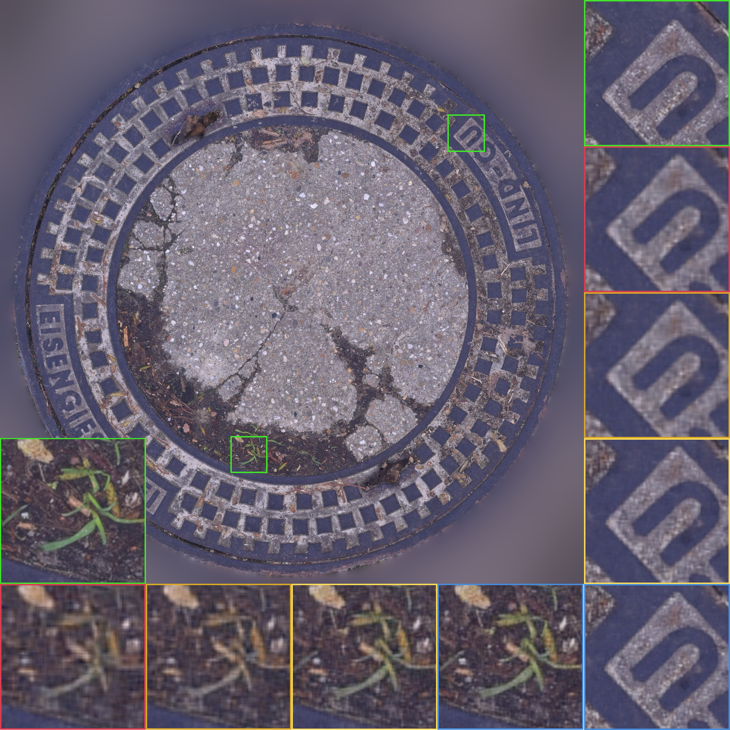
The MLP is learning to predict all the textures from the material set. The compression benefits come from the fact that a single .ntc can be used for all the textures of a model at the same time, since they are spatially correlated. Therefore for the comparisons to make sense, the reference is the sum size of all the textures in the material set. The original textures are .png and the normal map takes 21MB which is 57% of the whole set. The comparison with this texture set favors the NTC, as it includes 7 textures in a lossless format. In Table 1, the compression rate includes all the textures in the material set, but the PSNR values are of the albedo only.
| mip | resolution | reference | low |
medium |
high |
veryHigh |
|---|---|---|---|---|---|---|
.ntc size |
- | 36.54 MB | 0.72 MB | 1.3 MB | 2.81 MB | 4.98 MB |
| compression ratio vs PNG | - | 1× | 50.7x | 28.1x | 13.0x | 7.3x |
| 0 | 2048² | - | 26.67 | 27.56 | 29.40 | 30.95 |
| 1 | 1024² | - | 30.13 | 31.82 | 33.45 | 34.55 |
| 2 | 512² | - | 32.43 | 32.47 | 31.19 | 32.14 |
| 3 | 256² | - | 27.57 | 28.56 | 30.28 | 32.74 |
| 4 | 128² | - | 31.37 | 33.22 | 36.34 | 39.89 |
| 5 | 64² | - | 35.51 | 36.20 | 38.02 | 39.02 |
| 6 | 32² | - | 32.59 | 35.63 | 39.00 | 42.19 |
| 7 | 16² | - | 39.71 | 41.78 | 40.21 | 43.98 |
| 8 | 8² | - | 41.02 | 45.06 | 36.21 | 45.75 |
| 9 | 4² | - | 40.00 | 44.34 | 41.15 | 48.40 |
| 10 | 2² | - | 29.89 | 27.79 | 30.60 | 29.33 |
| 11 | 1² | - | 30.42 | 28.57 | 27.57 | 30.46 |
NTCRenderer
The NTCRenderer is a submodule that renders a model using .ntc of different settings. The Flight Helmet consists of 5 meshes and each mesh has its own .ntc to decode as seen in Figure 7. The renderer uses PBR shading to showcase the compressed PBR materials.
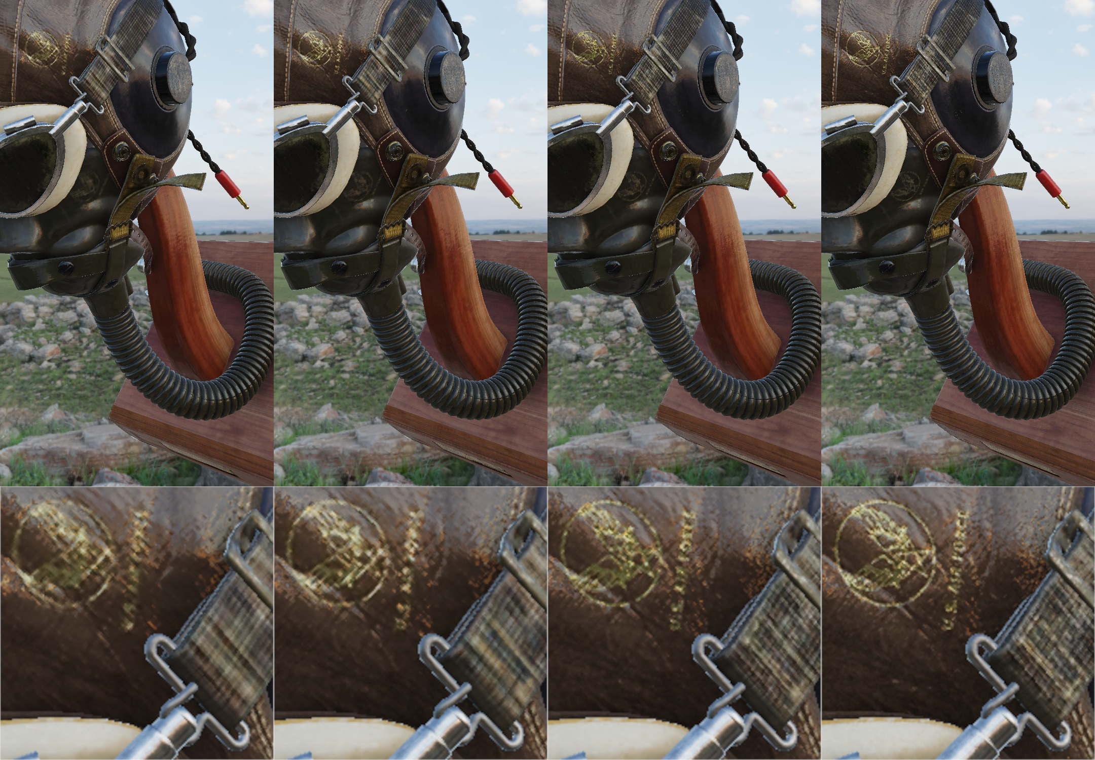
In that renderer there is also a version that infers a fullscreen texture and is used for benchmarking (Table 2), since every pixel on the screen is NTC inference.
| Device | Decode path | Inference @ 1920×1080 |
|---|---|---|
| M1 Air (cold, unthrottled) | half4 GEMV, per fragment |
51 ms |
| M5 Pro (20-core) | half4 GEMV, per fragment |
8.65 ms |
| M5 Pro (20-core) | tensor ops, 64 pixels per matmul | 1.96 ms |
With the neural accelerators, it is 4.4x faster than regular ALU. The M1 Air at 51ms puts real-time inference out of reach there. But the optimizations on that path are not wasted work, as it is the fallback for every non M5 and later machine. Whether it is usable on something like an M4 Max is untested.
NTC cost is scene-dependent
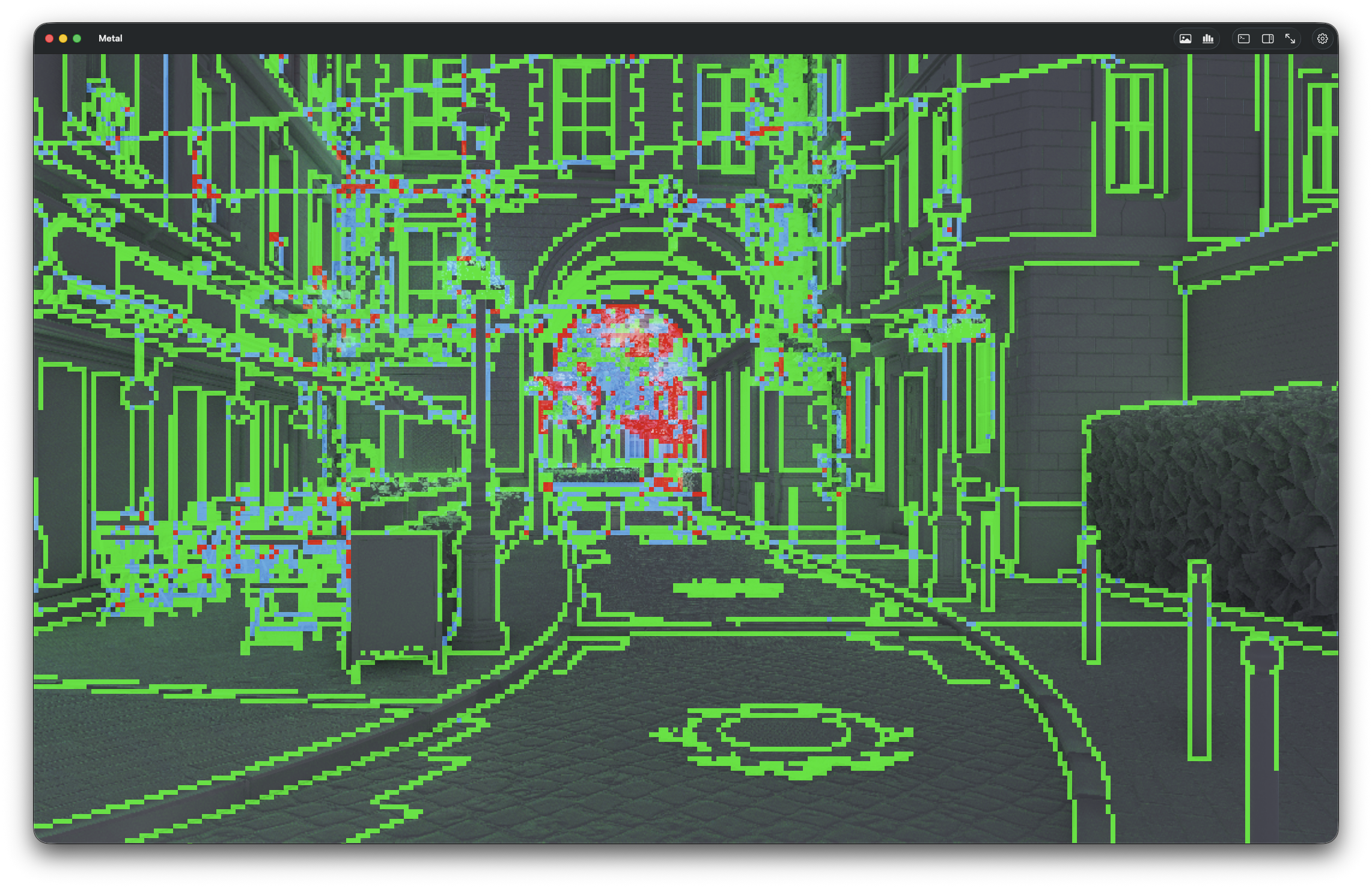
The fullscreen texture that was used in the benchmark does not reflect the real cost of NTC inference. On the same system when running the Bistro scene at 1920x1080p the inference costs around 3.6ms. That can be explained by the many different .ntc buffers that need to be decoded, texture targets that the specific pass needs to write for later stages in the pipeline and cache misses. In Figure 8 it shows the tiles that are made of 4 simdgroups, having to access only its own material which shows as grey, 2 materials as green, 3 materials as blue and 4 or more materials as red. When that happens, the tile runs the matmul once per material, over all 64 of its rows, keeping only the rows belonging to that material. It also has to reach a second latent pyramid in device memory, which is likely to cost cache misses, though I didn’t measure that.
Latency hiding
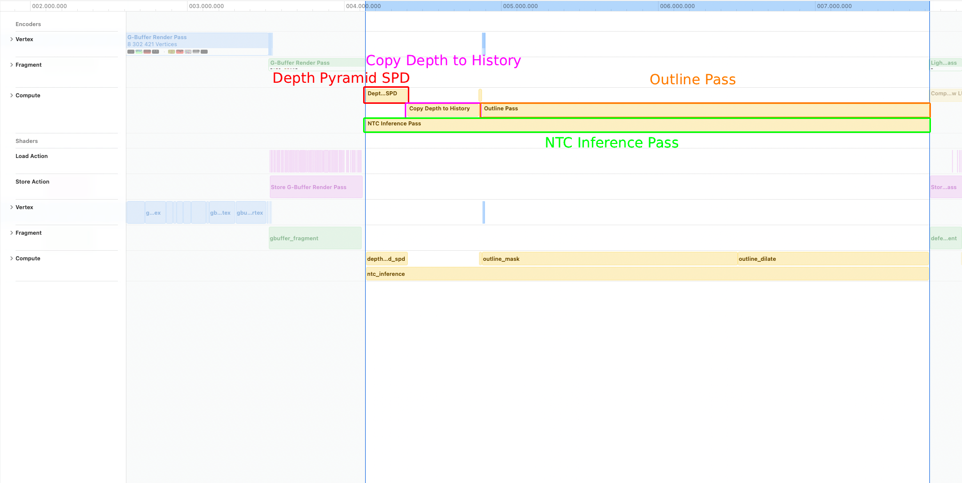
Stages that do not depend on the NTC can run concurrently with it and hide part of the inference cost. In Figure 9, the depth pyramid, copy depth to history and the outline pass (which is used for my editor) overlap the inference. None of them read the G-buffer targets the decode writes, so Metal schedules them alongside it automatically. Since NTC inference is using the neural accelerators, the ALUs are largely free for other passes.
Discussion
Room for experimentation
Real-time inference seems to be viable for systems that have neural accelerators. Currently the quality settings affect only the storage, but in the future I want to experiment with different configurations which will affect both storage and inference performance, like decreasing the features per latent grid texel. For just inference performance, lowering the hidden layer size could be tried. In general there is a lot of room for experimentation regarding performance.
On-load instead of inference
For systems that don’t have neural accelerators like the M1 Air, NTC could still be used to save disk storage but not VRAM. The models can store the .ntc files and on the engine start up, the .ntc will be decoded into textures for texture sampling. However by using the .ntc storage, it automatically means that the textures will be lossy like jpeg. The compression against jpeg materials is less impressive over the 7.3x compression on veryHigh settings that Table 1 shows.
Anisotropic filtering
Anisotropic filtering is not feasible in MetalNTC currently. It is the same shape of problem that Stochastic Trilinear Filtering solves, trade many taps for one plus a temporal resolve, but the footprint of anisotropic filtering is longer. For that reason I didn’t try solving anisotropy stochastically as the accumulator would need many more frames to converge, where it would break under fast motion. I believe the correct path to solve anisotropy for NTC is to bake it during training.
Where NTC can’t replace texture sampling
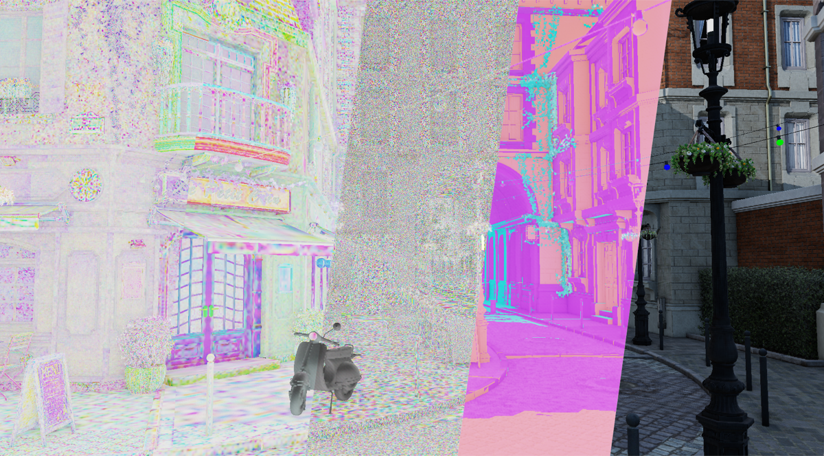
NTC can’t entirely replace texture sampling. The MLP emits every output channel in one evaluation, so there is no way to ask for a single one. Sampling just a displacement map costs the same as decoding the full texture set. And because the decode runs as a compute pass (with neural acceleration) after the G-buffer, anything needed earlier in the frame cannot use it at all. Alpha testing has to decide whether to discard a fragment while it is being rasterized, before the decode. NTC therefore needs to work alongside traditional texture sampling. Texture sampling can also be preferable when a mesh’s materials have different resolutions, since one .ntc covers a whole texture set at a single latent grid resolution. This is the case of the vespa in Bistro, visible in the title image. I skip neural textures entirely for such meshes. It could be resolved by upscaling the lower resolution materials of the texture set to the highest, but it did not seem worth the hassle, as such meshes rarely happen.
Source code
References
- Random-Access Neural Compression of Material Textures
- RTXNTC
- Metal Shading Language Specification
- Running inline ML operations in a shader with Metal 4
- Metal Performance Primitives (MPP) Programming Guide
- ADAM: A METHOD FOR STOCHASTIC OPTIMIZATION
- Amazon Lumberyard. Amazon Lumberyard Bistro, Open Research Content Archive (ORCA), July 2017.